An Introduction to Machine Learning and Its Applications: A Visual Tutorial
BY NICK MCCREA – SOFTWARE ENGINEER @ TOPTAL (link to original article)
Machine Learning (ML) is coming into its own, with a growing recognition that ML can play a key role in a wide range of critical applications, such as data mining, natural language processing, image recognition, and expert systems. ML provides potential solutions in all these domains and more, and is set to be a pillar of our future civilization.
The supply of able ML designers has yet to catch up to this demand. A major reason for this is that ML is just plain tricky. This tutorial introduces the basics of Machine Learning theory, laying down the common themes and concepts, making it easy to follow the logic and get comfortable with the topic.

What is Machine Learning?
So what exactly is “machine learning” anyway? ML is actually a lot of things. The field is quite vast and is expanding rapidly, being continually partitioned and sub-partitioned ad nauseam into different sub-specialties and types of machine learning.
There are some basic common threads, however, and the overarching theme is best summed up by this oft-quoted statement made by Arthur Samuel way back in 1959: “[Machine Learning is the] field of study that gives computers the ability to learn without being explicitly programmed.”
And more recently, in 1997, Tom Mitchell of Carnegie Mellon University gave a “well-posed” definition that has proven more useful to engineering types: “A computer program is said to learn from experience E with respect to some task T and some performance measure P, if its performance on T, as measured by P, improves with experience E.”
So if you want your program to predict, for example, traffic patterns at a busy intersection (task T), you can run it through a machine learning algorithm with data about past traffic patterns (experience E) and, if it has successfully “learned”, it will then do better at predicting future traffic patterns (performance measure P).
The highly complex nature of many real-world problems, though, often means that inventing specialized algorithms that will solve them perfectly every time is impractical, if not impossible. Examples of machine learning problems include, “Is this cancer?”, “What is the market value of this house?”, “Which of these people are good friends with each other?”, “Will this rocket engine explode on take off?”, “Will this person like this movie?”, “Who is this?”, “What did you say?”, and “How do you fly this thing?”. All of these problems are excellent targets for an ML project, and in fact ML has been applied to each of them with great success.
Among the different types of ML tasks, a crucial distinction is drawn between supervised and unsupervised learning:
- Supervised machine learning: The program is “trained” on a pre-defined set of “training examples”, which then facilitate its ability to reach an accurate conclusion when given new data.
- Unsupervised machine learning: The program is given a bunch of data and must find patterns and relationships therein.
We will primarily focus on supervised learning here, but the end of the article includes a brief discussion of unsupervised learning with some links for those who are interested in pursuing the topic further.
Supervised Machine Learning
In the majority of supervised learning applications, the ultimate goal is to develop a finely tuned predictor function h(x) (sometimes called the “hypothesis”). “Learning” consists of using sophisticated mathematical algorithms to optimize this function so that, given input data x about a certain domain (say, square footage of a house), it will accurately predict some interesting value h(x) (say, market price for said house).
In practice, x almost always represents multiple data points. So, for example, a housing price predictor might take not only square-footage (x1) but also number of bedrooms (x2), number of bathrooms (x3), number of floors (x4), year built (x5), zip code (x6), and so forth. Determining which inputs to use is an important part of ML design. However, for the sake of explanation, it is easiest to assume a single input value is used.
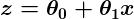
So let’s say our simple predictor has this form:
where θ0 and θ1 are constants. Our goal is to find the perfect values of θ0 and θ1 to make our predictor work as well as possible.
Optimizing the predictor h(x) is done using training examples. For each training example, we have an input value x_train, for which a corresponding output, y, is known in advance. For each example, we find the difference between the known, correct value y, and our predicted value h(x_train). With enough training examples, these differences give us a useful way to measure the “wrongness” of h(x). We can then tweak h(x) by tweaking the values of θ0 and θ1 to make it “less wrong”. This process is repeated over and over until the system has converged on the best values for θ0 and θ1. In this way, the predictor becomes trained, and is ready to do some real-world predicting.
A Simple Machine Learning Example
We stick to simple problems in this post for the sake of illustration, but the reason ML exists is because, in the real world, the problems are much more complex. On this flat screen we can draw you a picture of, at most, a three-dimensional data set, but ML problems commonly deal with data with millions of dimensions, and very complex predictor functions. ML solves problems that cannot be solved by numerical means alone.
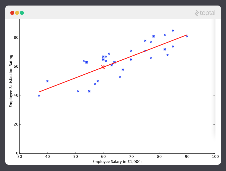
With that in mind, let’s look at a simple example. Say we have the following training data, wherein company employees have rated their satisfaction on a scale of 1 to 100:
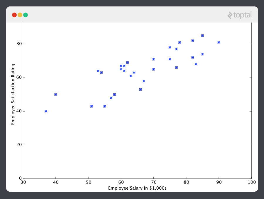
First, notice that the data is a little noisy. That is, while we can see that there is a pattern to it (i.e. employee satisfaction tends to go up as salary goes up), it does not all fit neatly on a straight line. This will always be the case with real-world data (and we absolutely want to train our machine using real-world data!). So then how can we train a machine to perfectly predict an employee’s level of satisfaction? The answer, of course, is that we can’t. The goal of ML is never to make “perfect” guesses, because ML deals in domains where there is no such thing. The goal is to make guesses that are good enough to be useful.
It is somewhat reminiscent of the famous statement by British mathematician and professor of statistics George E. P. Box that “all models are wrong, but some are useful”.
ML builds heavily on statistics. For example, when we train our machine to learn, we have to give it a statistically significant random sample as training data. If the training set is not random, we run the risk of the machine learning patterns that aren’t actually there. And if the training set is too small (see law of large numbers in Wikipedia, or law of large numbers that’s web-accessible), we won’t learn enough and may even reach inaccurate conclusions. For example, attempting to predict company-wide satisfaction patterns based on data from upper management alone would likely be error-prone.
With this understanding, let’s give our machine the data we’ve been given above and have it learn it. First we have to initialize our predictor h(x) with some reasonable values of θ0 and θ1. Now our predictor looks like this when placed over our training set:
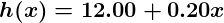

If we ask this predictor for the satisfaction of an employee making $60k, it would predict a rating of 27:
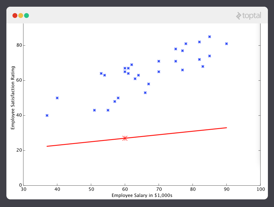
It’s obvious that this was a terrible guess and that this machine doesn’t know very much.
So now, let’s give this predictor all the salaries from our training set, and take the differences between the resulting predicted satisfaction ratings and the actual satisfaction ratings of the corresponding employees. If we perform a little mathematical wizardry (which I will describe shortly), we can calculate, with very high certainty, that values of 13.12 for θ0 and 0.61 for θ1 are going to give us a better predictor.
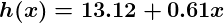
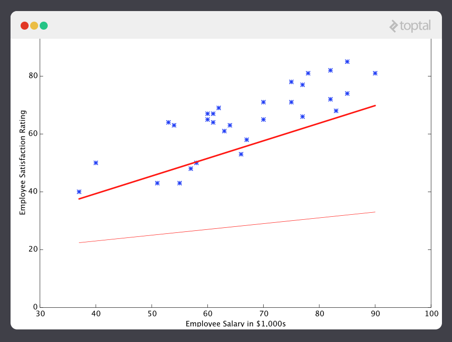
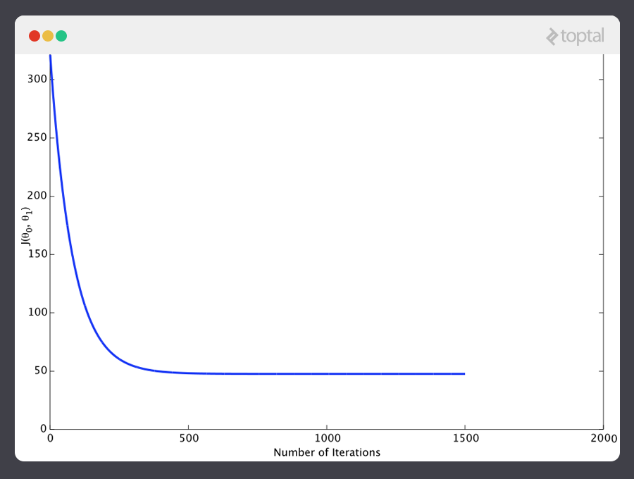
And if we repeat this process, say 1500 times, our predictor will end up looking like this:
At this point, if we repeat the process, we will find that θ0 and θ1 won’t change by any appreciable amount anymore and thus we see that the system has converged. If we haven’t made any mistakes, this means we’ve found the optimal predictor. Accordingly, if we now ask the machine again for the satisfaction rating of the employee who makes $60k, it will predict a rating of roughly 60.
Now we’re getting somewhere.
A Note on Complexity
The above example is technically a simple problem of univariate linear regression, which in reality can be solved by deriving a simple normal equation and skipping this “tuning” process altogether. However, consider a predictor that looks like this:

This function takes input in four dimensions and has a variety of polynomial terms. Deriving a normal equation for this function is a significant challenge. Many modern machine learning problems take thousands or even millions of dimensions of data to build predictions using hundreds of coefficients. Predicting how an organism’s genome will be expressed, or what the climate will be like in fifty years, are examples of such complex problems.
Fortunately, the iterative approach taken by ML systems is much more resilient in the face of such complexity. Instead of using brute force, a machine learning system “feels its way” to the answer. For big problems, this works much better. While this doesn’t mean that ML can solve all arbitrarily complex problems (it can’t), it does make for an incredibly flexible and powerful tool.
Gradient Descent – Minimizing “Wrongness”
Let’s take a closer look at how this iterative process works. In the above example, how do we make sure θ0 and θ1 are getting better with each step, and not worse? The answer lies in our “measurement of wrongness” alluded to previously, along with a little calculus.
The wrongness measure is known as the cost function (a.k.a., loss function), J(θ0,θ1). The input θ represents all of the coefficients we are using in our predictor. So in our case, θ is really the pair θ0 and θ1. J(θ0,θ1) gives us a mathematical measurement of how wrong our predictor is when it uses the given values of θ0 and θ1.
The choice of the cost function is another important piece of an ML program. In different contexts, being “wrong” can mean very different things. In our employee satisfaction example, the well-established standard is the linear least squares function:
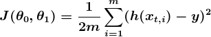
With least squares, the penalty for a bad guess goes up quadratically with the difference between the guess and the correct answer, so it acts as a very “strict” measurement of wrongness. The cost function computes an average penalty over all of the training examples.
So now we see that our goal is to find θ0 and θ1 for our predictor h(x) such that our cost function J(θ0,θ1) is as small as possible. We call on the power of calculus to accomplish this.
Consider the following plot of a cost function for some particular ML problem:
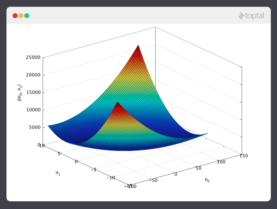
Here we can see the cost associated with different values of θ0 and θ1. We can see the graph has a slight bowl to its shape. The bottom of the bowl represents the lowest cost our predictor can give us based on the given training data. The goal is to “roll down the hill”, and find θ0 and θ1 corresponding to this point.
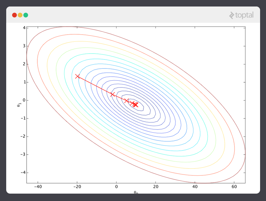
This is where calculus comes in to this machine learning tutorial. For the sake of keeping this explanation manageable, I won’t write out the equations here, but essentially what we do is take the gradient of J(θ0,θ1), which is the pair of derivatives of J(θ0,θ1) (one over θ0 and one over θ1). The gradient will be different for every different value of θ0 and θ1, and tells us what the “slope of the hill is” and, in particular, “which way is down”, for these particular θs. For example, when we plug our current values of θ into the gradient, it may tell us that adding a little to θ0 and subtracting a little from θ1 will take us in the direction of the cost function-valley floor. Therefore, we add a little to θ0, and subtract a little from θ1, and voilà! We have completed one round of our learning algorithm. Our updated predictor, h(x) = θ0 + θ1x, will return better predictions than before. Our machine is now a little bit smarter.
This process of alternating between calculating the current gradient, and updating the θs from the results, is known as gradient descent.
That covers the basic theory underlying the majority of supervised Machine Learning systems. But the basic concepts can be applied in a variety of different ways, depending on the problem at hand.
Classification Problems
Under supervised ML, two major subcategories are:
- Regression machine learning systems: Systems where the value being predicted falls somewhere on a continuous spectrum. These systems help us with questions of “How much?” or “How many?”.
- Classification machine learning systems: Systems where we seek a yes-or-no prediction, such as “Is this tumer cancerous?”, “Does this cookie meet our quality standards?”, and so on.
As it turns out, the underlying theory is more or less the same. The major differences are the design of the predictor h(x) and the design of the cost function J(θ).
Our examples so far have focused on regression problems, so let’s now also take a look at a classification example.
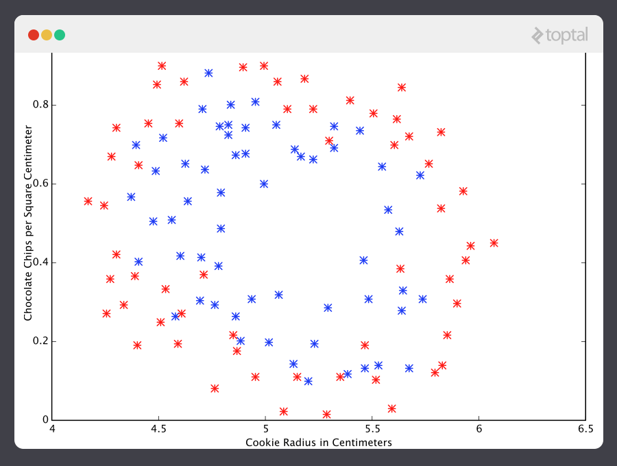
Here are the results of a cookie quality testing study, where the training examples have all been labeled as either “good cookie” (y = 1) in blue or “bad cookie” (y = 0) in red.
In classification, a regression predictor is not very useful. What we usually want is a predictor that makes a guess somewhere between 0 and 1. In a cookie quality classifier, a prediction of 1 would represent a very confident guess that the cookie is perfect and utterly mouthwatering. A prediction of 0 represents high confidence that the cookie is an embarrassment to the cookie industry. Values falling within this range represent less confidence, so we might design our system such that prediction of 0.6 means “Man, that’s a tough call, but I’m gonna go with yes, you can sell that cookie,” while a value exactly in the middle, at 0.5, might represent complete uncertainty. This isn’t always how confidence is distributed in a classifier but it’s a very common design and works for purposes of our illustration.
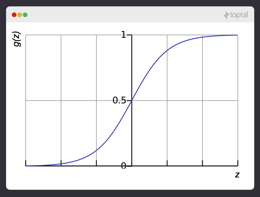
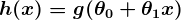
It turns out there’s a nice function that captures this behavior well. It’s called the sigmoid function, g(z), and it looks something like this:
z is some representation of our inputs and coefficients, such as:
so that our predictor becomes:
Notice that the sigmoid function transforms our output into the range between 0 and 1.
The logic behind the design of the cost function is also different in classification. Again we ask “what does it mean for a guess to be wrong?” and this time a very good rule of thumb is that if the correct guess was 0 and we guessed 1, then we were completely and utterly wrong, and vice-versa. Since you can’t be more wrong than absolutely wrong, the penalty in this case is enormous. Alternatively if the correct guess was 0 and we guessed 0, our cost function should not add any cost for each time this happens. If the guess was right, but we weren’t completely confident (e.g. y = 1, but h(x) = 0.8), this should come with a small cost, and if our guess was wrong but we weren’t completely confident (e.g. y = 1 but h(x) = 0.3), this should come with some significant cost, but not as much as if we were completely wrong.
This behavior is captured by the log function, such that:
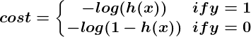
Again, the cost function J(θ) gives us the average cost over all of our training examples.
So here we’ve described how the predictor h(x) and the cost function J(θ) differ between regression and classification, but gradient descent still works fine.
A classification predictor can be visualized by drawing the boundary line; i.e., the barrier where the prediction changes from a “yes” (a prediction greater than 0.5) to a “no” (a prediction less than 0.5). With a well-designed system, our cookie data can generate a classification boundary that looks like this:
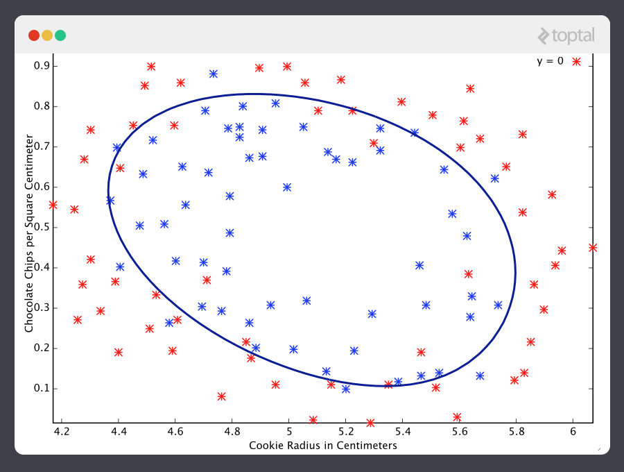
Now that’s a machine that knows a thing or two about cookies!
An Introduction to Neural Networks
No discussion of ML would be complete without at least mentioning neural networks. Not only do neural nets offer an extremely powerful tool to solve very tough problems, but they also offer fascinating hints at the workings of our own brains, and intriguing possibilities for one day creating truly intelligent machines.
Neural networks are well suited to machine learning problems where the number of inputs is gigantic. The computational cost of handling such a problem is just too overwhelming for the types of systems we’ve discussed above. As it turns out, however, neural networks can be effectively tuned using techniques that are strikingly similar to gradient descent in principle.
A thorough discussion of neural networks is beyond the scope of this tutorial, but I recommend checking out our previous post on the subject.
Unsupervised Machine Learning
Unsupervised learning typically is tasked with finding relationships within data. There are no training examples used in this process. Instead, the system is given a set data and tasked with finding patterns and correlations therein. A good example is identifying close-knit groups of friends in social network data.
The algorithms used to do this are very different from those used for supervised learning, and the topic merits its own post. However, for something to chew on in the meantime, take a look at clustering algorithms such as k-means, and also look into dimensionality reduction systems such as principle component analysis. Our prior post on big data discusses a number of these topics in more detail as well.
Conclusion
We’ve covered much of the basic theory underlying the field of Machine Learning here, but of course, we have only barely scratched the surface.
Keep in mind that to really apply the theories contained in this introduction to real life machine learning examples, a much deeper understanding of the topics discussed herein is necessary. There are many subtleties and pitfalls in ML, and many ways to be lead astray by what appears to be a perfectly well-tuned thinking machine. Almost every part of the basic theory can be played with and altered endlessly, and the results are often fascinating. Many grow into whole new fields of study that are better suited to particular problems.
Clearly, Machine Learning is an incredibly powerful tool. In the coming years, it promises to help solve some of our most pressing problems, as well as open up whole new worlds of opportunity. The demand for ML engineers is only going to continue to grow, offering incredible chances to be a part of something big. I hope you will consider getting in on the action!
Acknowledgement
This article draws heavily on material taught by Stanford Professor Dr. Andrew Ng in his free and open Machine Learning course. The course covers everything discussed in this article in great depth, and gives tons of practical advice for the ML practitioner. I cannot recommend this course highly enough for those interested in further exploring this fascinating field.
Nicholas is a professional software engineer with a passion for quality craftsmanship. He loves architecting and writing top-notch code, and is proud of his ability to synthesize and communicate ideas effectively to technical and non-technical folks alike. Nicholas always enjoys a novel challenge.